This page presents statistics of solar irradiance monitoring stations using data from SolarStations.org.
import pandas as pd
import matplotlib.pyplot as plt
import matplotlib.ticker as ticker
import numpy as np
from datetime import datetime as dt
from IPython.display import Markdown as md
from matplotlib.lines import Line2D
df = pd.read_csv('./SolarStationsOrg-station-catalog.csv')
# make different colors based on stations status
df['color'] = 'red'
df['color'] = df['color'].mask(df['Time period'].str.endswith('-'), 'green').mask(df['Time period'].str.endswith('?'), 'blue')
# Define start operation period
df['start'] = None
df.loc[df['Time period'].str.len()>1, 'start'] = df['Time period'].str[:4]
df['start'] = df['start'].astype(pd.Int64Dtype())
# Define end operation period
df['end'] = None
df.loc[df['Time period'].str.len()==9, 'end'] = df['Time period'].str[5:]
df.loc[df['Time period'].str.len()==4, 'end'] = df['Time period']
df['end'] = df['end'].astype(pd.Int64Dtype())dfs = df.copy().set_index('Station name')
# Drop stations with unknown time period ('?' or '')
dfs = dfs[dfs['start'].notna()]
dfs.loc[dfs['end'].isna(), 'end'] = pd.Timestamp.today().year
# Drop stations with only one year of data
dfs = dfs[dfs['start'] != dfs['end']]
# Sort the dataframe based on the start operation date and station status (color)
dfs = dfs.sort_values(['start', 'color'], ascending=False)
dfs = dfs.reset_index()fig, ax = plt.subplots(figsize=(6, 3))
ax.barh(dfs.index, dfs['end']-dfs['start'], left=dfs['start'], color=dfs['color'], zorder=2)
ax.set_yticks([])
ax.set_title('History of station status')
ax.set_xticks(np.arange(1970,dt.today().year+5,5))
ax.set_xlim(1975,dt.today().year+1)
ax.grid(alpha=0.5, zorder=-1)
plt.figtext(0.5, -0.03, 'Station start and end year.', wrap=True, horizontalalignment='center', fontsize=9)
# custom legend
custom_lines = [Line2D([0], [0], color='green', lw=4),
Line2D([0], [0], color='blue', lw=4),
Line2D([0], [0], color='red', lw=4)]
ax.legend(custom_lines, ['Active', 'Unknown', 'Inactive']);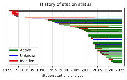
Let’s take a closer look at the current active stations and their measurement records.
active_stations_count = df.loc[df['color']=='green', 'start'].value_counts().sort_index()

fig, axes = plt.subplots(figsize=(6, 3))
axes.plot(active_stations_count.cumsum())

axes.set_ylabel('Number of active stations [-]')
axes.grid(alpha=0.5)
axes.set_xticks(np.arange(1970, dt.today().year+5, 5))
axes.set_xlim(1975, dt.today().year+1)
axes.set_ylim(0, np.ceil((active_stations_count.cumsum().max()+3)/50)*50)
plt.figtext(0.5, -0.03, 'Active stations available for each year.',
            wrap=True, horizontalalignment='center', fontsize=9)
plt.show()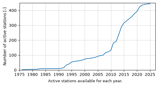
a = df.loc[df['color']=='green']
year = 1993
stations_before_year = len(a.loc[a['start']<year])
percent_before_year = round(1-(len(a)-len(a.loc[a['start']<year]))/len(a),3)*100
total_active = len(a)

last_20_years = dt.today().year - 20
stations_last_20_years = len(a.loc[a['start']>last_20_years])
percent_last_20_years = round(1-(len(a)-len(a.loc[a['start']>last_20_years]))/len(a),3)*100

df['Unknown_status'] = df['Time period'].str.endswith('?')
dfu = df.loc[df['Unknown_status']]
md(f'The following conclusions can be drawn from the figures above: \n'
f'* There are currently {total_active} active stations out of the {df.shape[0]} known stations\n'
f'* Of the active stations, only {stations_before_year} have been in operation before {year} (~{percent_before_year:.0f}%) \n'
f'* Most of the active stations ({stations_last_20_years}) have been in operation for less than 20 years (~{int(percent_last_20_years)}%) \n'
f'* There are {len(dfu)} stations ({len(dfu)/df.shape[0]*100:.0f}%) whose operation status is unknown, which demonstrates a huge barrier to accessing information and data from solar stations!'
)Dataset duration
The figure below provides an overview of the operation duration of the active and inactive stations.
# use only active and inactive stations (remove unknown status)
df_known = df.loc[df['color'].isin(['green','red'])].copy()
# find the operation years for each station
df_known['operation_years'] = df_known['end'].fillna(pd.Timestamp.today().year).subtract(df_known['start'])
step_size = 5
bins = np.arange(0, df_known['operation_years'].max()+step_size, step_size)
fig, ax = plt.subplots(figsize=(4, 2.5))
df_known.loc[:, 'operation_years'].hist(
ax=ax, bins=bins, zorder=2, color='red', label='Inactive',
edgecolor='black', linewidth=0.4)
df_known.loc[df_known['color']=='green', 'operation_years'].hist(
ax=ax, bins=bins, zorder=2, color='green', label='Active',
edgecolor='black', linewidth=0.4)
ax.set_ylabel('Total number of stations')
ax.grid(alpha=0.5, which='both', axis='y', zorder=-1)
ax.set_xlabel('Operating years')
ax.set_title('Dataset length')
ax.set_xlim(0, None)
ax.legend(loc='upper right')
plt.show()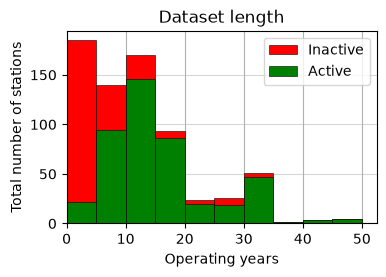
The graph shows that most of the stations with measurement record greater than 15 years remain in operation.
Historical and active stations
# Top 15 countries
countries = df.groupby('Country').count()['Station name'].sort_values(ascending=False)[:15]
# Plot
fig, axes = plt.subplots(figsize=(4, 2.5))
countries.plot.bar(zorder=2, width=0.3, edgecolor='black', linewidth=0.4)
axes.set_ylabel('Total number of stations')
axes.set_ylim(0, countries.iloc[0]+5)
axes.set_yticks(np.arange(0,countries.iloc[0]+20,20))
axes.grid(alpha=0.5, which='both', axis='y', zorder=-1)
axes.set_xlabel('')
plt.show()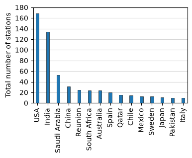
print('List of historical and active networks:')
df['Network'].str.replace(' ','').str.split(';', expand=True).stack().value_counts()
List of historical and active networks:
SRRA                                                    123
ESMAP                                                    91
BSRN                                                     78
WEST                                                     52
NOAA                                                     39
IOS-net                                                  37
SAURAN                                                   22
MIDC                                                     17
QEERI                                                    15
BOM                                                      15
AEMET                                                    14
WMORRC                                                   14
FONDEF                                                   13
SMHI                                                     12
enerMENA                                                 10
SURFRAD                                                  10
WMOGAW                                                   10
SOLRAD                                                    9
PPA                                                       8
SRML                                                      7
CBSRN                                                     7
RMCIS                                                     6
SONDA                                                     6
SKYNET                                                    6
DOERTC                                                    6
ARAD                                                      5
SEMRTS                                                    4
IMS                                                       4
ABO                                                       4
ARM                                                       4
HBCU                                                      3
AERONET                                                   3
NRELMIDC                                                  3
CHOPIN                                                    2
LithuanianHydrometeorologicalService(LHMS)                2
LatvianEnvironmentGeologyandMeteorologyCentre(LEGMC)      1
ARG/AcademyofSciencesofMoldova                            1
GAW-WMO                                                   1
SlovakHydrometeorologicalInstitute                        1
IDMP                                                      1
Name: count, dtype: int64
# Stations per KG climate zone
# Break down the station into Tier
climate_zone = df.groupby(['Koeppen Geiger climate zone','Tier']).count()['Station name'].unstack('Tier').fillna(0)
# Find the total number of stations (Tier 1 + Tier 2)
climate_zone['sum'] = climate_zone[1.0] + climate_zone[2.0]
# Sort the dataframe from high number of stations to low
climate_zone.sort_values(by='sum', ascending=False, inplace=True)
# drop the 'sum' column for easier plotting
climate_zone.drop(columns='sum', inplace=True)
climate_zone.columns = climate_zone.columns.astype(int)
# plot
fig, axes = plt.subplots(figsize=(4, 2.5))
climate_zone.plot.bar(ax=axes, zorder=2, width=0.3, rot=0, stacked=True,
edgecolor='black', linewidth=0.4)
axes.set_ylim(0, climate_zone.iloc[0][1]+climate_zone.iloc[0][2]+5)
axes.set_yticks(np.arange(0,climate_zone.iloc[0][1]+climate_zone.iloc[0][2]+50,50))
axes.grid(alpha=0.5, which='both', axis='y', zorder=-1)
axes.set_ylabel('Total number of stations')
axes.set_xlabel('')
plt.xticks(rotation=45)
plt.show()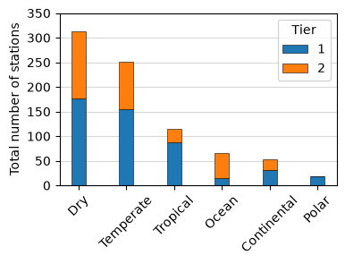
Zooming in on active stations
The remainder of the plots and statistics will be based only on the Active stations.
# create a column indicating if a station is active
df['Active'] = df['Time period'].str.endswith('-')
# create a new dataframe containing only the active stations

# REMOVE THE ==True WHEN THERE ARE NO NAN VALUES
dfa = df.loc[df['Active']==True]
print(f'The number of active stations: {len(dfa)}')
The number of active stations: 447
Station tier
The figure below shows the percentage of active stations categorized as either Tier 1 or Tier 2. It can be observed that most of the active stations are Tier 1, which means that they measure global horizontal irradiance (GHI), diffuse horizontal irradiance (DHI) using a shadow ball, and direct normal irradiance (DNI) using a pyrheliometer mounted on a solar tracker. For more information on the station tier classifications, see the station requirements page.
# Station tier
tier_rename = {1: 'Tier 1', 2: 'Tier 2'}

fig, axes = plt.subplots(figsize=(3, 3))
dfa['Tier'].map(tier_rename).convert_dtypes().value_counts().\
    plot.pie(autopct='%1.0f%%', explode=[0, 0.1],
             wedgeprops = {'linewidth': 0.3, 'edgecolor': 'black'})
axes.set_ylabel('')
axes.set_title('Station tier');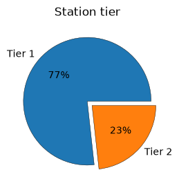
Leading countries
The figure below shows the number of active stations for the top 5 countries.
# Break down the station into Tier
countries_tier_active = dfa.groupby(['Country','Tier']).count()['Station name'].unstack('Tier').fillna(0)
# Find the total number of stations (Tier 1 + Tier 2)
countries_tier_active['sum'] = countries_tier_active[1] + countries_tier_active[2]
# Sort the dataframe from high number of stations to low
countries_tier_active.sort_values(by='sum', ascending=False, inplace=True)
# drop the 'sum' column for easier plotting
countries_tier_active.drop(columns='sum', inplace=True)

# plot
fig, axes = plt.subplots(figsize=(4, 2.5))
countries_tier_active[:5].plot.bar(ax=axes, zorder=2, width=0.3, rot=0, stacked=True,
                                  edgecolor='black', linewidth=0.4)  # plot only the top 5 countries
axes.set_yticks(np.arange(0, countries_tier_active.iloc[0][1]+countries_tier_active.iloc[0][2]+10, 10))
axes.grid(alpha=0.5, which='both', axis='y', zorder=-1)
axes.set_ylabel('Number of active stations')
axes.set_xlabel('')
axes.set_title('Top 5 countries')
plt.figtext(0.5, -0.03, 'Top five countries with the most active stations.', wrap=True, horizontalalignment='center', fontsize=9);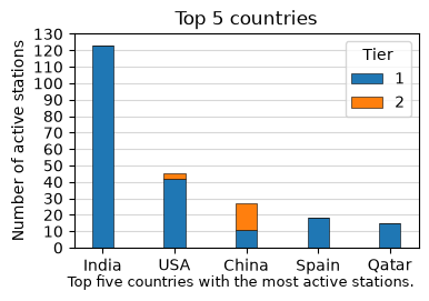
networks = dfa['Network'].str.replace(' ','').str.split(';', expand=True).stack().value_counts()

md(f"Most of the active stations belong to a network, which makes their data easier to access (partly because they usually have a website):\n"
   f'* {networks.index[0]} : {networks.iloc[0]} \n'
   f'* {networks.index[1]} : {networks.iloc[1]} \n'
   f'* {networks.index[2]} : {networks.iloc[2]} \n'
   f'* {networks.index[3]} : {networks.iloc[3]} \n'
   f'* {networks.index[4]} : {networks.iloc[4]} \n'
   f'* {networks.index[5]} : {networks.iloc[5]} \n'
   f'* {networks.index[6]} : {networks.iloc[6]} \n'
   f'* {networks.index[7]} : {networks.iloc[7]} \n'
   f'* {networks.index[8]} : {networks.iloc[8]} \n'
   f'* {networks.index[9]} : {networks.iloc[9]} \n'
   f'* {networks.index[10]} : {networks.iloc[10]} \n'
)Breakdown by continent and climate
continents = dfa.groupby('Continent').count().sort_values(by='Continent')['Station name']
continents
Continent
Africa 73
Antarctica 6
Asia 215
Europe 74
North America 59
Oceania 9
South America 11
Name: Station name, dtype: int64fig, axes = plt.subplots(figsize=(3, 3))
autopct = lambda x: '{:.0f}'.format(x * continents.sum() / 100)
pie = axes.pie(continents, autopct=autopct, pctdistance=0.85, startangle=34,
explode=np.ones(7)*0.05,
wedgeprops = {'linewidth': 0.3, 'edgecolor': 'black'})
axes.legend(continents.index, loc=2, bbox_to_anchor=(1,0.75), frameon=False)
axes.set_title('Active stations per continent');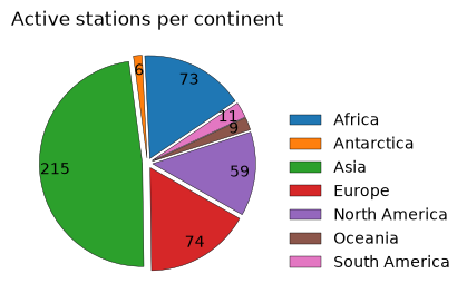
# plt.rcParams.update({'font.size': 7}) # increase the font size of the x and y axis

# continents.index = ['Africa', 'Antarctica', 'Asia', 'Europe', 'N. America', 'Oceania', 'S. America']

# fig, axes = plt.subplots(figsize=(3, 2.5))

# autopct = lambda x: '{:.0f}'.format(x * continents.sum() / 100)

# continents.plot.bar(zorder=2, edgecolor='k', linewidth=0.5, rot=40)
# axes.set_yticks(np.arange(0,221,20))
# axes.set_ylim(0,220)
# axes.grid(alpha=0.5, which='both', axis='y', zorder=-1)
# axes.set_ylabel('Number of active stations')
# axes.set_xlabel('')
# plt.savefig('C:/Users/iosif/Dropbox (Personal)/Apps/Overleaf/solar_stations/figures/statistics.png', bbox_inches='tight', dpi=600)
# ;
# land areas of contients per km^2 from Wikipedia
continent_area={
'Asia':44614000,
'Africa':30365000,
'North America':24230000,
'South America':17814000,
'Antarctica':14200000,
'Europe':10000000,
'Oceania':8510926
}countries_continent_tier_active = dfa.groupby(['Continent','Tier']).count()['Station name'].unstack('Tier').fillna(0)
station_per_km = pd.DataFrame(dtype='float64')
for i in continents.index:
station_per_km[i] = countries_continent_tier_active.loc[i]/continent_area[i]*1000000 # this is stations per Tm^2
station_per_km = station_per_km.T
# Find the total number of stations (Tier 1 + Tier 2)
station_per_km['sum'] = station_per_km[1] + station_per_km[2]
# Sort the dataframe from high number of stations to low
station_per_km.sort_values(by='sum', ascending=False, inplace=True)
# drop the 'sum' column for easier plotting
station_per_km.drop(columns='sum', inplace=True)fig, axes = plt.subplots(figsize=(4, 2.5))
station_per_km.plot.bar(ax=axes, zorder=2, width=0.3, rot=90, stacked=True,
edgecolor='black', linewidth=0.4)
axes.set_yticks(np.arange(0,station_per_km.iloc[0][1.0]+station_per_km.iloc[0][2.0]+1,1))
axes.grid(alpha=0.5, which='both', axis='y', zorder=-1)
axes.set_ylabel('Active stations per million km$^2$')
axes.set_xlabel('')
axes.set_title('Geographical coverage by continent');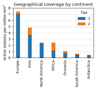
# Stations per KG climate zone
# Break down the station into Tier
climate_zone = dfa.groupby(['Koeppen Geiger climate zone','Tier']).count()['Station name'].unstack('Tier').fillna(0)
# Find the total number of stations (Tier 1 + Tier 2)
climate_zone['sum'] = climate_zone[1.0] + climate_zone[2.0]
# Sort the dataframe from high number of stations to low
climate_zone.sort_values(by='sum', ascending=False, inplace=True)
# drop the 'sum' column for easier plotting
climate_zone.drop(columns='sum', inplace=True)
fig, axes = plt.subplots(figsize=(4, 2.5))
climate_zone.plot.bar(ax=axes, zorder=2, width=0.3, rot=0, stacked=True,
edgecolor='black', linewidth=0.4)
axes.set_ylim(0, climate_zone.iloc[0][1.0]+climate_zone.iloc[0][2.0]+5)
axes.grid(alpha=0.5, which='both', axis='y', zorder=-1)
axes.set_ylabel('Number of active stations')
axes.set_xlabel('')
axes.set_xticklabels(axes.get_xticklabels(), rotation=45, ha='right')
axes.set_title('Stations by Köppen–Geiger climate zone')
plt.show()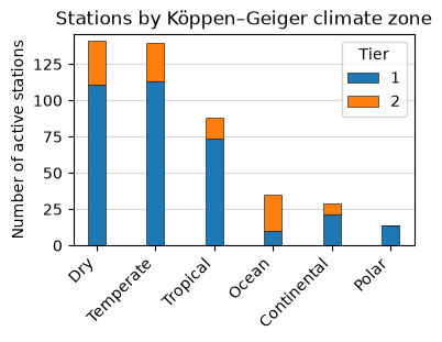
Breakdown by elevation and latitude
stations_per_500m = dfa.groupby(pd.cut(dfa['Elevation'], np.arange(0, 5000, 500)), observed=False)['Station name'].count()

fig, axes = plt.subplots(figsize=(4, 2.5))
stations_per_500m.plot.bar(zorder=2, edgecolor='black', linewidth=0.4)
axes.set_yticks(np.arange(0, stations_per_500m[1]+50, 50))
axes.grid(alpha=0.5, which='both', axis='y', zorder=-1)
axes.set_ylabel('Number of active stations')
axes.set_xlabel('Elevation [m]')
axes.set_title('Stations categorized by elevation');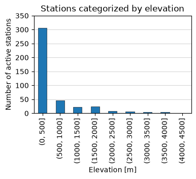
stations_per_10deg = dfa.groupby(pd.cut(dfa['Latitude'], np.arange(-90, 90+10, 10)), observed=False)['Station name'].count()

fig, axes = plt.subplots(figsize=(4, 2.5))
stations_per_10deg.plot.bar(zorder=2, edgecolor='black', linewidth=0.4)
axes.set_yticks(np.arange(0, stations_per_10deg.max()+10, 15))
axes.grid(alpha=0.5, which='both', axis='y', zorder=-1)
axes.set_ylabel('Number of active stations')
axes.set_xlabel('Latitude [°]')
axes.set_title('Stations categorized by latitude');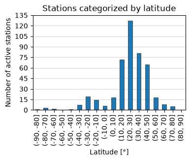
Components
This section is not active -- requires more careful analysis.
component_dict = {
    'G': 'GHI',
    'D': 'DHI',
    'B': 'DNI',
}

components = dfa['Instrumentation'].str.split(';', expand=True).stack().value_counts()

fig, axes = plt.subplots(figsize=(4, 2.5))
components.plot.bar(zorder=2, edgecolor='black', linewidth=0.4)
axes.set_yticks(np.arange(0,components.iloc[0]+50,50))
axes.grid(alpha=0.5, which='both', axis='y', zorder=-1)
axes.set_ylabel('Number of active stations')
axes.set_title('Irradiance components measured');
components
G 372
B 363
D 347
IR 96
UV 43
SPN1 27
Ds 17
PAR 16
RSI 5
RSR 4
GTI 3
Albedo 2
UVA 1
UVB 1
albedo 1
Name: count, dtype: int64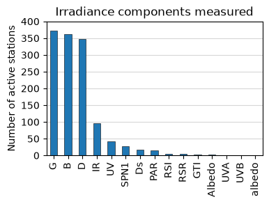
Data availability
df_un = dfa[(dfa['Data availability'].isna()) | (dfa['Data availability']=='Not available')]
df_av = dfa[(dfa['Data availability']=='Freely') | (dfa['Data availability']=='Free')]
df_req = dfa[dfa['Data availability']=='Upon request']
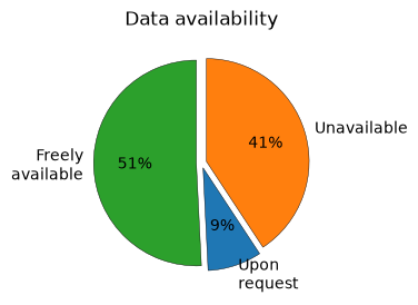
md(f'Finding and downloading data from solar stations can be a tedious process. The main reason is that often there is no information on how to obtain the data. '
f'There are {len(df_av)} active stations where data can be freely donwloaded and {len(df_un)} stations for which there is no data access. The figure shows the corresponding percentages.')fig, axes = plt.subplots(figsize=(3, 3))
axes.pie([len(df_av), len(df_req), len(df_un)], labels=['Freely\navailable','Upon\nrequest','Unavailable'],
colors=['C2','C0','C1'], autopct='%1.0f%%', startangle=90,
explode=[0.05, 0.05, 0.05],
wedgeprops = {'linewidth': 0.3, 'edgecolor': 'black'})
axes.set_title('Data availability');